Calibration workflow

Packages

For the complete workflow, data.table and ggplot2 are required besides envalysis.

library(envalysis)
library(data.table)
library(ggplot2)

Sample data

The sample data used stems from Steinmetz et al. (2019). It consists of two tables: a sequence table and a sample table.

The sequence table contains gas-chromatography/mass spectrometry measurement data of two phenolic compounds, these are tyrosol and vanillin. Besides the samples, standard mixtures and extraction blanks (type) were acquired in three separate analysis batches. Each measurement resulted in an integrated peak area.

Compound	Type	Batch	Name	Area	Spec Conc
Tyrosol	Extraction blank	1	Blank 1	0.000000	NA
Tyrosol	Extraction blank	1	Blank 2	0.000000	NA
Tyrosol	Sample	1	ZS-001	328.343597	NA
Tyrosol	Sample	1	ZS-002	282.930939	NA
Tyrosol	Standard	3	0 mg/L	0.000000	0.00000
Tyrosol	Standard	3	1 mg/L	7.628456	0.97755
Tyrosol	Standard	3	5 mg/L	35.566628	4.88775
Tyrosol	Standard	3	20 mg/L	141.898056	19.55100
Tyrosol	Standard	3	100 mg/L	715.496338	97.75500
Vanillin	Sample	1	ZS-001	1876.933716	NA
Vanillin	Sample	1	ZS-002	1578.626099	NA

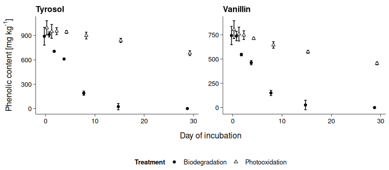
The sample table describes the samples’ origin from a 29-day degradation experiment, in which the phenolic compounds were either degraded in the dark by the native soil microbial community or photooxidized under UV irradiation after sterilizing the soil. The samples were processed in threefold replication. Their weight [g], the volume [mL] of extract solution, and the dilution factor were recorded.

Name	Day	Lighting	Sterilization	Treatment	Replicate	Weight	Extract	Dilution
ZS-001	0	UV	sterilized	Photooxidation	1	2.5037	12.5	5
ZS-002	0	UV	sterilized	Photooxidation	2	2.5018	12.5	5
ZS-019	0	dark	non-sterilized	Biodegradation	1	2.5001	12.5	5
ZS-164	29	dark	non-sterilized	Biodegradation	2	2.4992	12.5	1
ZS-165	29	dark	non-sterilized	Biodegradation	3	2.5000	12.5	1

In envalysis, the sample data is stored in a two-item list called phenolics. The list items are named seq and samples.

data("phenolics")
str(phenolics)

# > List of 2
# >  $ seq    :'data.frame':    160 obs. of  6 variables:
# >   ..$ Compound : Factor w/ 2 levels "Tyrosol","Vanillin": 1 1 1 1 1 1 1 1 1 1 ...
# >   ..$ Type     : Factor w/ 3 levels "Extraction blank",..: 1 1 2 2 2 2 2 2 2 2 ...
# >   ..$ Batch    : int [1:160] 1 1 1 1 1 1 1 1 1 1 ...
# >   ..$ Name     : chr [1:160] "Blank 1" "Blank 2" "ZS-001" "ZS-002" ...
# >   ..$ Area     : num [1:160] 0 0 328 283 296 ...
# >   ..$ Spec Conc: num [1:160] NA NA NA NA NA NA NA NA NA NA ...
# >  $ samples:'data.frame':    42 obs. of  9 variables:
# >   ..$ Name         : chr [1:42] "ZS-001" "ZS-002" "ZS-003" "ZS-019" ...
# >   ..$ Day          : int [1:42] 0 0 0 0 0 0 1 1 1 1 ...
# >   ..$ Lighting     : Factor w/ 2 levels "dark","UV": 2 2 2 1 1 1 2 2 2 1 ...
# >   ..$ Sterilization: Factor w/ 2 levels "non-sterilized",..: 2 2 2 1 1 1 2 2 2 1 ...
# >   ..$ Treatment    : Factor w/ 2 levels "Biodegradation",..: 2 2 2 1 1 1 2 2 2 1 ...
# >   ..$ Replicate    : int [1:42] 1 2 3 1 2 3 1 2 3 1 ...
# >   ..$ Weight       : num [1:42] 2.5 2.5 2.5 2.5 2.5 ...
# >   ..$ Extract      : num [1:42] 12.5 12.5 12.5 12.5 12.5 12.5 12.5 12.5 12.5 12.5 ...
# >   ..$ Dilution     : int [1:42] 5 5 5 5 5 5 2 2 2 2 ...

Simple calibation

Since the two phenolic compounds were analyzed in three different batches, six individual calibration curves are required for quantification. For better understanding, the calibration workflow is first shown for a subset of data, namely the first batch of tyrosol measurements. The subset is stored in tyrosol_1.

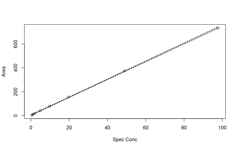
All standards in the tyrosol_1 subset are used for calibration. The 'calibration' object is stored as cal_1, which can be printed for additional information including limits of detection and quantification, the adjusted R², blanks, and statistical checks of the underlying calibration model.

tyrosol_1 <- subset(phenolics$seq, Compound == "Tyrosol" & Batch == 1)

cal_1 <- calibration(Area ~ `Spec Conc`,
                     data = subset(tyrosol_1, Type == "Standard"))

print(cal_1)

# > 
# > Call:
# > calibration(formula = Area ~ `Spec Conc`, data = subset(tyrosol_1, 
# >     Type == "Standard"))
# > 
# > Coefficients:
# > (Intercept)  `Spec Conc`  
# >       3.762        7.508  
# > 
# > Adjusted R-squared:  0.9998
# > Sum relative error:  1.558
# > 
# > Blanks:
# > [1] 0.07470126 0.06534690 0.06093782 0.00000000
# > 
# >     `Spec Conc`     lwr     upr
# > LOD      0.0144 0.00952  0.0293
# > LOQ      5.9300 3.92000 12.1000
# > 
# > Check for normality of residuals:
# > 
# >     Shapiro-Wilk normality test
# > 
# > data:  residuals(calibration(formula = Area ~ `Spec Conc`, data = subset(tyrosol_1, )residuals(    Type == "Standard")))
# > W = 0.87897, p-value = 0.1841
# > 
# > Check for homoscedasticity of residuals:
# > 
# >     studentized Breusch-Pagan test
# > 
# > data:  Area ~ `Spec Conc`
# > BP = 0.40323, df = 1, p-value = 0.5254

plot(cal_1)

Based on cal_1, the tyrosol concentrations can be calculated for all samples using inv_predict(). The argument below_lod = 0 specifies that concentrations below limit of detection (LOD) should be set to zero.

tyrosol_1$`Calc Conc` <- inv_predict(cal_1, tyrosol_1$Area, below_lod = 0)
head(tyrosol_1)

# >   Compound             Type Batch    Name     Area Spec Conc Calc Conc
# > 1  Tyrosol Extraction blank     1 Blank 1   0.0000        NA   0.00000
# > 2  Tyrosol Extraction blank     1 Blank 2   0.0000        NA   0.00000
# > 3  Tyrosol           Sample     1  ZS-001 328.3436        NA  43.23037
# > 4  Tyrosol           Sample     1  ZS-002 282.9309        NA  37.18195
# > 5  Tyrosol           Sample     1  ZS-003 296.2863        NA  38.96072
# > 6  Tyrosol           Sample     1  ZS-019 243.0258        NA  31.86707

Working with `data.table`s

To process all compounds and analysis batches together, the phenolics data is converted to data.tables.

dt <- lapply(phenolics, as.data.table)

To replicate the following steps, try to organize your data in the same way as shown before. If you want to read in your data directly as data.table, use their fread() function, for instance.

Batch calibration

Subsequently, calibration() and inv_predict() are applied by compound and batch.

dt$seq[, `Calc Conc` := calibration(Area ~ `Spec Conc`, .SD[Type == "Standard"]) |> 
         inv_predict(Area, below_lod = 0),
       by = .(Compound, Batch)]
head(dt$seq)

# >    Compound             Type Batch    Name     Area Spec Conc Calc Conc
# >      <fctr>           <fctr> <int>  <char>    <num>     <num>     <num>
# > 1:  Tyrosol Extraction blank     1 Blank 1   0.0000        NA   0.00000
# > 2:  Tyrosol Extraction blank     1 Blank 2   0.0000        NA   0.00000
# > 3:  Tyrosol           Sample     1  ZS-001 328.3436        NA  43.23037
# > 4:  Tyrosol           Sample     1  ZS-002 282.9309        NA  37.18195
# > 5:  Tyrosol           Sample     1  ZS-003 296.2863        NA  38.96072
# > 6:  Tyrosol           Sample     1  ZS-019 243.0258        NA  31.86707

Calibration parameters like LODs, LOQs, or adjusted R² may be stored in a separate list item for later use.

dt$cal <- dt$seq[Type == "Standard", calibration(Area ~ `Spec Conc`) |> 
                   as.list(c("coef", "adj.r.squared", "lod", "loq")),
                 by = .(Compound, Batch)]
print(dt$cal)

# >    Compound Batch (Intercept) `Spec Conc` adj.r.squared       lod       loq
# >      <fctr> <int>       <num>       <num>         <num>     <num>     <num>
# > 1:  Tyrosol     1  3.76202803    7.508184     0.9997915 0.0143933  5.925273
# > 2:  Tyrosol     2  3.07268449    7.601129     0.9992824 0.0092660 10.909912
# > 3:  Tyrosol     3  0.05587782    7.309053     0.9999764 0.0000000  2.311322
# > 4: Vanillin     1 25.17794786   51.529670     0.9998175 0.0040133  5.623778
# > 5: Vanillin     2 24.44314369   51.774820     0.9992359 0.0003509 11.408191
# > 6: Vanillin     3 10.62899985   50.819997     0.9999641 0.0000000  2.886073

Similarly, predict() may be used for plotting calibration curves independently of the plot() function.

dt$pred <- dt$seq[Type == "Standard", calibration(Area ~ `Spec Conc`) |> 
                    predict(),
                 by = .(Compound, Batch)]
head(dt$pred)

# >    Compound Batch Spec.Conc       fit      lwr      upr
# >      <fctr> <int>     <num>     <num>    <num>    <num>
# > 1:  Tyrosol     1 0.4887750  7.431840 3.504021 11.35966
# > 2:  Tyrosol     1 0.6105099  8.345849 4.425043 12.26665
# > 3:  Tyrosol     1 0.7322449  9.259857 5.346040 13.17367
# > 4:  Tyrosol     1 0.8539798 10.173866 6.267011 14.08072
# > 5:  Tyrosol     1 0.9757148 11.087874 7.187956 14.98779
# > 6:  Tyrosol     1 1.0974497 12.001882 8.108875 15.89489

Blank subtraction

With the calculated concentrations at hand, the sample concentrations are subtracted by the extraction blanks to correct for potential lab-borne contamination.

dt$seq[, `Clean Conc` := `Calc Conc` - mean(
  `Calc Conc`[Type == "Extraction blank"], na.rm = T),
  by = .(Batch, Compound)]

Merging tables

The sequence table is merged with the sample table and the contents of phenolic compounds are calculated from the extraction volume, sample weight, and dilution factor.

dt$res <- merge(dt$seq, dt$samples, by = "Name")

dt$res[, Content := `Clean Conc` * (Extract / Weight) * Dilution]
head(dt$res)

# > Key: <Name>
# >      Name Compound   Type Batch      Area Spec Conc Calc Conc Clean Conc   Day
# >    <char>   <fctr> <fctr> <int>     <num>     <num>     <num>      <num> <int>
# > 1: ZS-001  Tyrosol Sample     1  328.3436        NA  43.23037   43.23037     0
# > 2: ZS-001 Vanillin Sample     1 1876.9337        NA  35.93572   35.93572     0
# > 3: ZS-002  Tyrosol Sample     1  282.9309        NA  37.18195   37.18195     0
# > 4: ZS-002 Vanillin Sample     1 1578.6261        NA  30.14667   30.14667     0
# > 5: ZS-003  Tyrosol Sample     1  296.2863        NA  38.96072   38.96072     0
# > 6: ZS-003 Vanillin Sample     1 1593.6272        NA  30.43779   30.43779     0
# >    Lighting Sterilization      Treatment Replicate Weight Extract Dilution
# >      <fctr>        <fctr>         <fctr>     <int>  <num>   <num>    <int>
# > 1:       UV    sterilized Photooxidation         1 2.5037    12.5        5
# > 2:       UV    sterilized Photooxidation         1 2.5037    12.5        5
# > 3:       UV    sterilized Photooxidation         2 2.5018    12.5        5
# > 4:       UV    sterilized Photooxidation         2 2.5018    12.5        5
# > 5:       UV    sterilized Photooxidation         3 2.5048    12.5        5
# > 6:       UV    sterilized Photooxidation         3 2.5048    12.5        5
# >      Content
# >        <num>
# > 1: 1079.1621
# > 2:  897.0653
# > 3:  928.8800
# > 4:  753.1246
# > 5:  972.1515
# > 6:  759.4865

Plotting

For plotting the data using ggplot2, the contents are summarized by mean and confidence interval (CI).

dt$sum <- dt$res[, .(Content = mean(Content, na.rm = T),
                     CI = CI(Content, na.rm = T)),
                 by = .(Compound, Treatment, Day)]

ggplot(dt$sum, aes(x = Day, y = Content)) +
  geom_errorbar(aes(ymin = Content - CI, ymax = Content + CI, group = Treatment),
                width = 1, position = position_dodge(1)) +
  geom_point(aes(shape = Treatment, fill = Treatment),
             position = position_dodge(1)) +
  xlab("Day of incubation") +
  ylab(expression("Phenolic content"~"["*mg~kg^-1*"]")) +
  facet_wrap(~ Compound, ncol = 2, scales = "free") +
  scale_shape_manual(values = c(21,24)) +
  scale_fill_manual(values = c("black", "white")) +
  theme_publish()

References

Steinmetz, Z., Kurtz, M.P., Zubrod, J.P., Meyer, A.H., Elsner, M., & Schaumann, G.E. (2019) Biodegradation and photooxidation of phenolic compounds in soil—A compound-specific stable isotope approach. Chemosphere 230, 210-218. DOI: 10.1016/j.chemosphere.2019.05.030.

Zacharias Steinmetz

2024-10-17

Packages

Sample data

Simple calibation

Working with `data.table`s

Batch calibration

Blank subtraction

Merging tables

Plotting

References

Calibration workflow

Zacharias Steinmetz

2024-10-17

Packages

Sample data

Simple calibation

Working with data.tables

Batch calibration

Blank subtraction

Merging tables

Plotting

References

Working with `data.table`s